API documentation
This section of the documentation details the auto-generated API from Read the Docs.
-
class
bioLEC.LEC.landscapeConnectivity(filename=None, XYZ=None, Z=None, dx=None, periodic=False, symmetric=False, sigmap=0.1, sigmav=None, diagonals=True, delimiter=' ', sl=-1000000.0, test=False)[source]¶ Bases:
objectLandscape elevational connectivity (LEC) quantifies the closeness of a site to all others with similar elevation. Such closeness is computed over a graph whose edges represent connections among sites and whose weights are proportional to the cost of spreading through patches at different elevation.
- Method:
- E. Bertuzzo et al., 2016: Geomorphic controls on elevational gradients of species richness - PNAS doi
Parameters: - filename (str) – CSV file name containing regularly spaced elevation grid [default: None]
- XYZ (3D Numpy Array) – 3D coordinates array of shape (nn,3) where nn is the number of points [default: None]
- Z (2D Numpy Array) – Elevation array of shape (nx,ny) where nx and ny are the number of points along the X and Y axis [default: None]
- dx (float) – grid spacing in metre when the Z argument defined above is used [default: None]
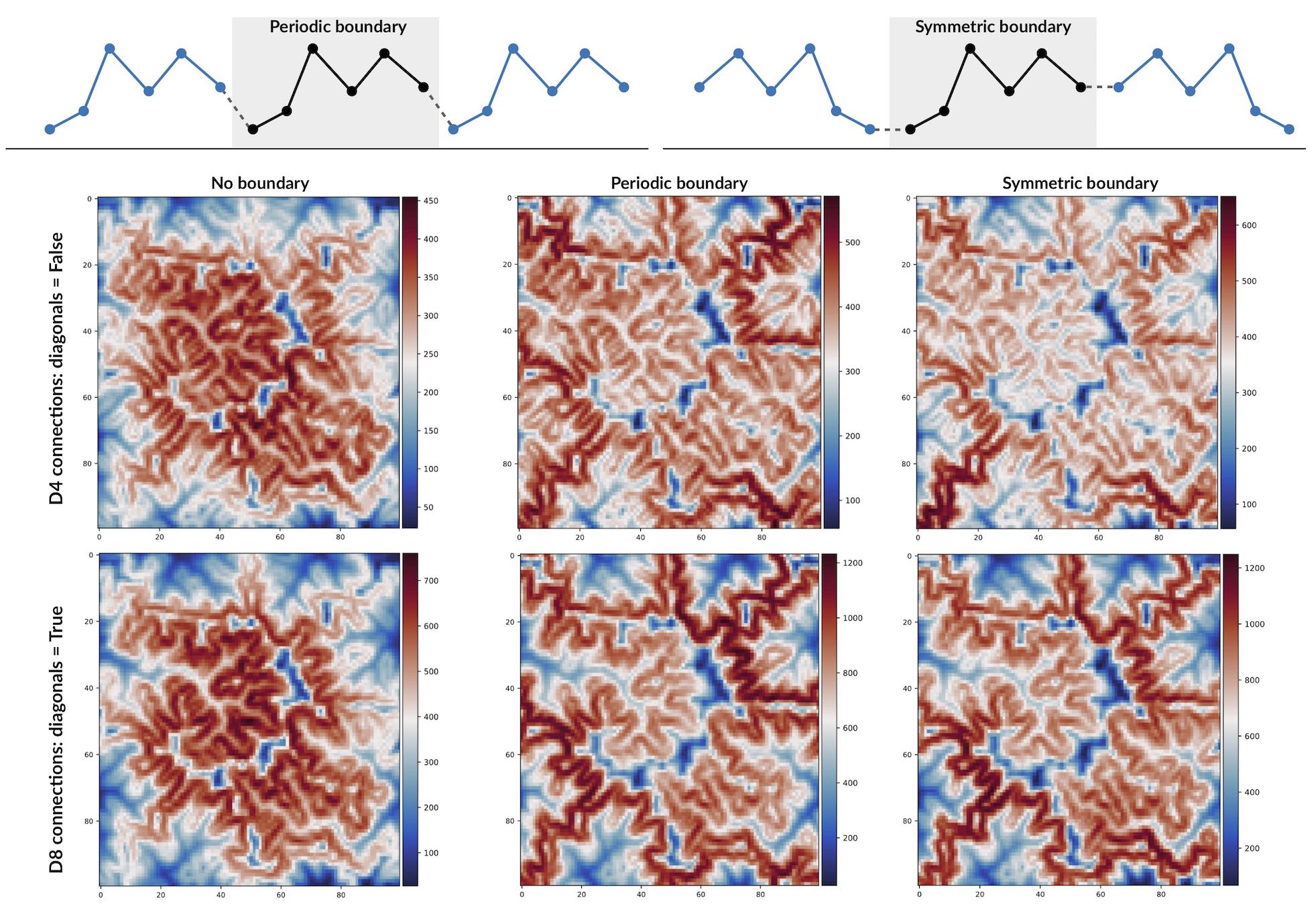
- periodic (bool) – applied periodic boundary to the elevation grid see explanation [default: False]
- symmetric (bool) – applied symmetric boundary to the elevation grid see explanation [default: False]
- sigmap (float) – species niche width percentage based on elevation extent [default: 0.1]
- sigmav (float) – species niche fixed width values [default: None]
- diagonals (bool) – computes the path based on the diagonal moves as well as the axial ones eg. D4/D8 connectivity [default: True]
- delimiter (str) – elevation grid csv delimiter [default: ‘ ‘]
- sl (float) – sea level position used to remove marine points from the LEC calculation [default: -1.e6]
Caution
There are 3 ways to import the elevation dataset in bioLEC:
- either as a CSV file (argument: filename) containing 3 columns for X, Y and Z respectively with no header and ordered along the X axis first
- or as a 3D numpy array (argument: XYZ) containing the X, Y and Z coordinates here again ordered along the X axis first
- or as a 2D numpy array (argument: Z) containing the elevation matrix, in this case the dx argument is also required
Note
It is worth noting that the boundary conditions are either symmetric or periodic. Although LEC simply depends on the elevation field and on the niche width, LEC predicts well the alpha-diversity simulated by full metacommunity models.
-
computeLEC(fout=500)[source]¶ This function computes the minimum path for all nodes in a given surface and measure of the closeness of each node to other at similar elevation range.
It then provide the landscape elevational connectivity array from computed measure of closeness calculation.
Parameters: fout (int) – output frequency [default: 500]
-
computeMinPath(r, c)[source]¶ Internal function to compute the minimum path between a specific node and all other ones.
Parameters: - c (int) – row indice of the consider point
- r (int) – column indice of a consider point
Returns: minimum-cost path for the specified node.
Return type: mincost
Note
This function relies on scikit-image (image processing in python) and finds distance-weighted minimum cost paths through an n-d costs array.
-
splitRowWise()[source]¶ Rowwise block partitioning used to perform LEC computation in parallel.
Returns: number of nodes to consider on each partition startID (1D array int): starting index for each partition endID (1D array int): ending index for each partition Return type: disps (1D array int) Note
From the number of processors (np) available split the array into equal number row wise.
-
viewElevFrequency(input=None, imName=None, nbins=80, size=(6, 6), fsize=11, dpi=200)[source]¶ This function plots and saves in a figure the distribution of elevation.
Parameters: - input (str) – CSV file name containing the dataset
- imName (str) – (string) image name with extension
- nbins (int) – number of bins for the histogram (default: 80)
- size – size of the image [default: (6,6)]
- fsize (int) – title font size [default: 11]
- dpi (int) – resolution of the saved image [default: 200]
Warning
The filename needs to be provided without extension.
-
viewLECFrequency(input=None, imName=None, size=(6, 6), fsize=11, dpi=200)[source]¶ This function plots and saves in a figure the distribution of LEC with elevation.
Parameters: - input (str) – CSV file name containing the dataset
- imName (str) – (string) image name with extension
- size – size of the image [default: (6,6)]
- fsize (int) – title font size [default: 11]
- dpi (int) – resolution of the saved image [default: 200]
Warning
The filename needs to be provided without extension.
-
viewLECZFrequency(input=None, imName=None, size=(6, 6), fsize=11, dpi=200)[source]¶ This function plots and saves in a figure the distribution of LEC and elevation with elevation.
Parameters: - input (str) – CSV file name containing the dataset
- imName (str) – (string) image name with extension
- size – size of the image [default: (6,6)]
- fsize (int) – title font size [default: 11]
- dpi (int) – resolution of the saved image [default: 200]
Warning
The filename needs to be provided without extension.
-
viewLECZbar(input=None, imName=None, nbins=40, size=(6, 6), fsize=11, dpi=200)[source]¶ This function plots and saves in a figure the distribution of LEC and elevation with elevation as well as the standard deviation for LEC values for each bins.
Parameters: - input (str) – CSV file name containing the dataset
- imName (str) – (string) image name with extension
- nbins (int) – number of bins for the histogram (default: 40)
- size – size of the image [default: (6,6)]
- fsize (int) – title font size [default: 11]
- dpi (int) – resolution of the saved image [default: 200]
Warning
The filename needs to be provided without extension.
-
viewResult(imName=None, size=(9, 5), fsize=11, cmap1=<matplotlib.colors.LinearSegmentedColormap object>, cmap2=<matplotlib.colors.LinearSegmentedColormap object>, dpi=200)[source]¶ This function plots and saves in a figure the result of the LEC computation.
Parameters: - imName (str) – (string) image name with extension
- size – size of the image [default: (9,5)]
- fsize (int) – title font size [default: 11]
- cmap1 – color map for elevation grid [default: plt.cm.summer_r]
- cmap2 – color map for LEC grid [default: cmap2=plt.cm.coolwarm]
- dpi (int) – resolution of the saved image [default: 200]
-
writeLEC(filename='LECout')[source]¶ This function writes the computed landscape elevational connectivity array in a CSV file and create a VTK visualisation file (.vts).
Parameters: filename (str) – output file name without format extension. Warning
The filename needs to be provided without extension.