What is the LEC?
LEC quantifies the closeness of a site to all others with similar elevation. For a given landscape, LEC is primarily dependent on elevation range and on species niche width. It quantifies the closeness of any point in the landscape to all others at similar elevation.
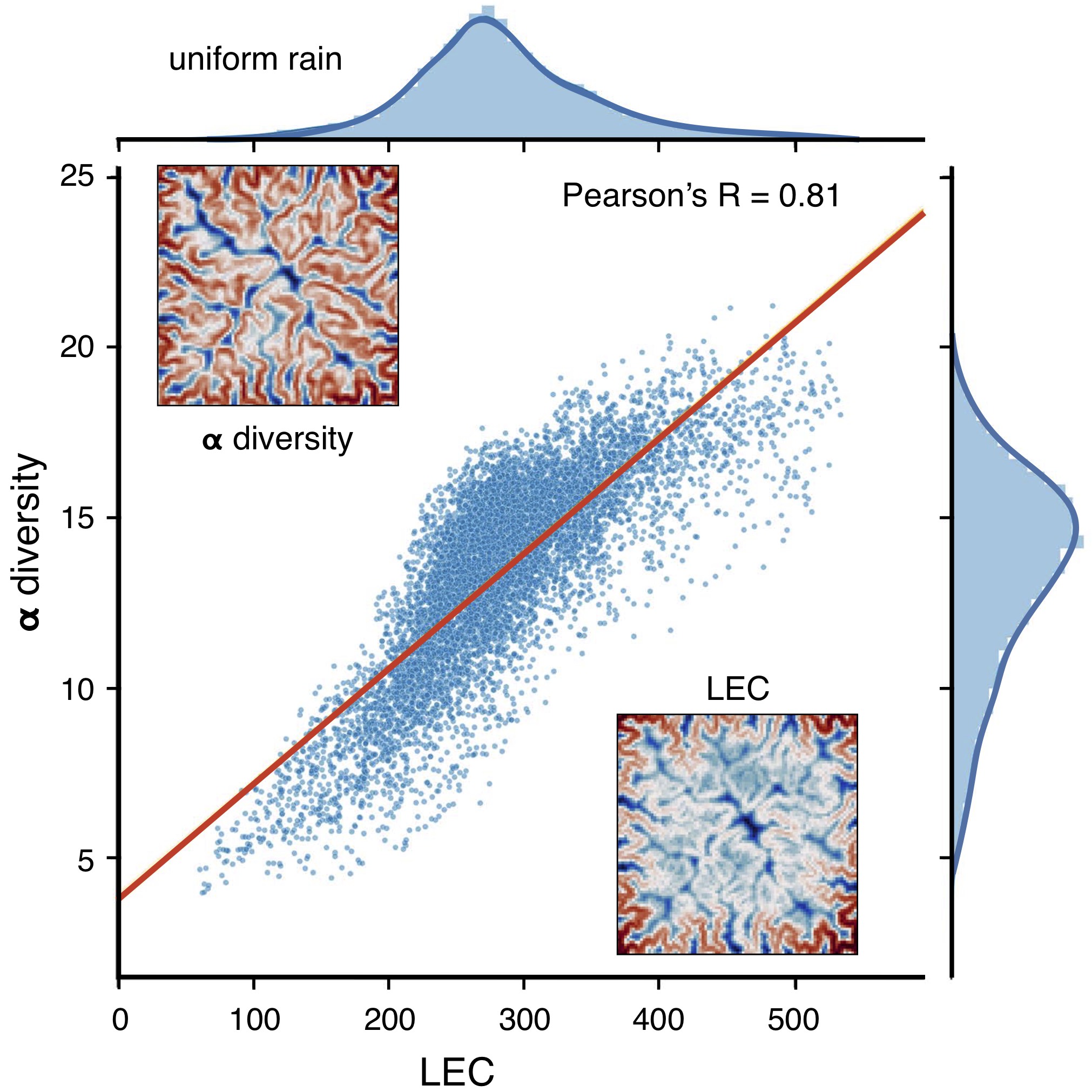
It has been shown that LEC captures well the \(\alpha\)-diversity variations observed in mountainous landscape [Lomolino2008] and simulated by full meta-community models [Bertuzzo2016] as shown in the figure below.
Important
It suggests that geomorphic features are a first-order control on biodiversity and that LEC metric can be used to quickly assess species richness distribution in complex landscapes.
Cost function
Considering a 2D lattice made of N squared cells, LEC for cell i (\({LEC}_i\)) is given by
where \(C_{ji}\) quantifies the closeness between sites j and i with respect to elevational connectivity. \(C_{ji}\) measures the cost for a given species adapted to cell j to spread and colonise cell i. This cost is a function of elevation and evaluates how often species adapted to the elevation of cell j have to travel outside their optimal species niche width (\(\sigma\)) to reach cell i (as shown in the figure below).
Following Bertuzzo et al. [Bertuzzo2016], \(C_{ji}\) is expressed as:
where \(p=[k_1,k_2, ...,k_L]\) (with \(k_1=j\) and \(k_L=i\)) are the cells comprised in the path p from j to i.
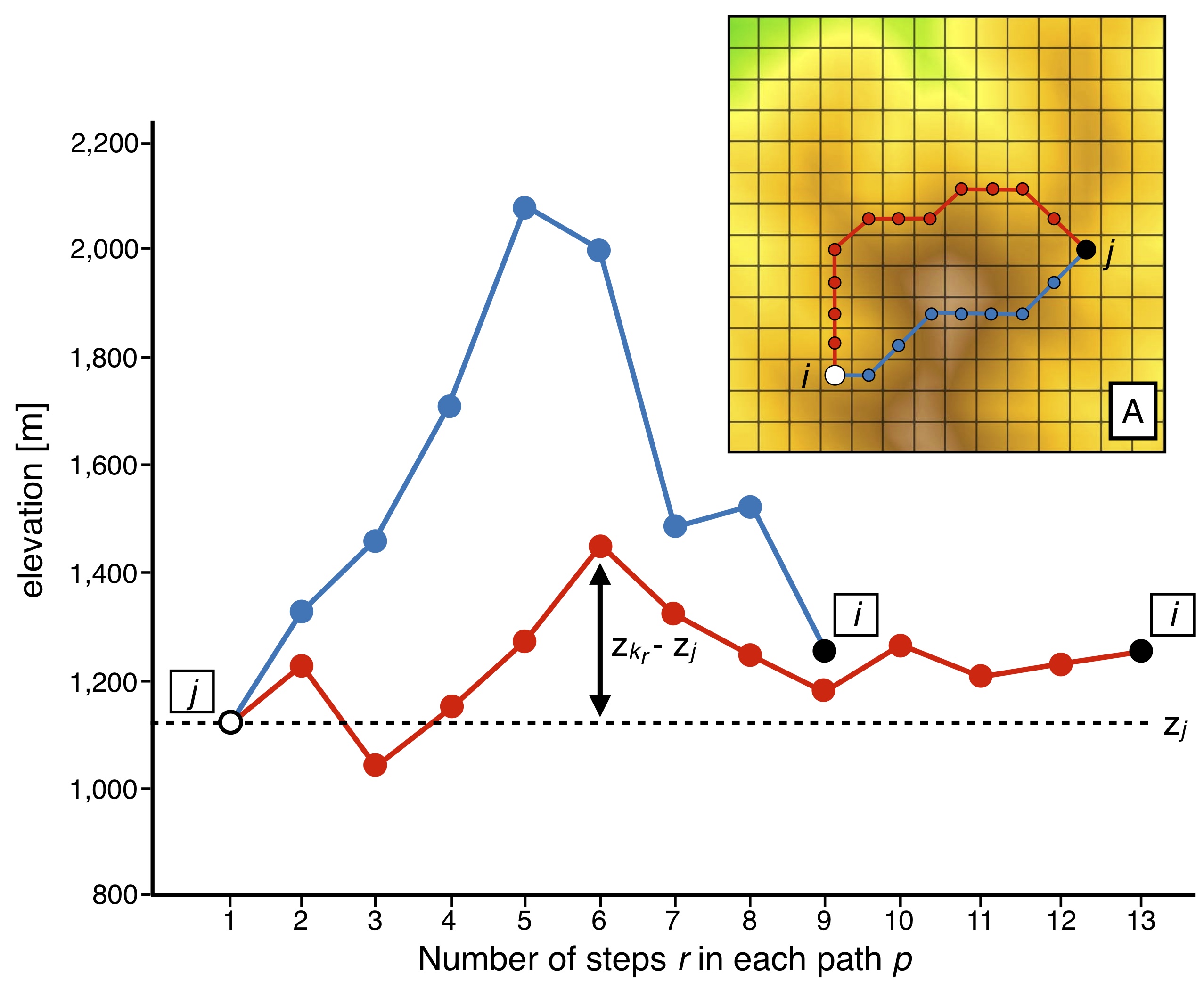
In the figure above, we illustrate the approach implemented in bioLEC to compute the closeness measure (\(C_{ji}\)) used to quantify LEC based on a topography grid (adapted from [Bertuzzo2016]). Two paths from site j to i (inset) are proposed with their elevation profiles. Associated costs are computed following the equation above (\(\sum_{r=2}^L (z_{k_r}-z_j)^2\)).
Hint
Despite a longer length, the cost associated to the red path is smaller than that of the blue one as it passes across sites with similar elevations to \(z_j\).
Dijkstra’s algorithm
The estimation of \(C_{ji}\) requires computation of all the possible paths p from j to i and is defined as the maximum closeness value along these paths and this is solved for each cell j using Dijkstra’s algorithm [Dijkstra1959] with diagonal connectivity between cells.
For each cell j, the algorithm builds a Dijkstra tree that branches the given cell with all the cells defining the simulated region. Edge weights are set equal to the square of the difference between the considered vertex elevation (\(z_{k_r}\)) and \(z_j\). The least-cost distance between j and i is then calculated as the minimum sum of edge weights obtained from the cells along the shortest-path (see top figure).
Here, the closeness is measured as a least-cost distances that optimises the costs associated to the edge weights of the traversed cells as well as the travelled Euclidean distance. As the least-cost distances incorporate landscape costs to movement, the approach allows for closeness differentiation between cells that might be seen as equally near if landscape costs were not accounted for.
In bioLEC we rely on scikit-image to compute the least cost distances [Etherington2017]. scikit-image package is primarily intended to process image [vanderWalt2014] but is designed to work with NumPy arrays making it compatible with other Python packages (e.g. most other geospatial Python packages) and really simple to use with digital elevation datasets.
While scikit-image uses slightly different terminology, talking about minimum cost paths rather than least-cost paths, the approach is identical to those commonly implemented in GIS software and applies Dijkstra’s algorithm with diagonal connectivity between cells [Etherington2016].
Parallelisation
Dijkstra’s algorithm is a graph search algorithm that solves single-source shortest path for a graph with non-negative weights. Such an algorithm can be quite long to solve especially in bioLEC as it needs to be used to compute the least-cost paths for every points on the surface.
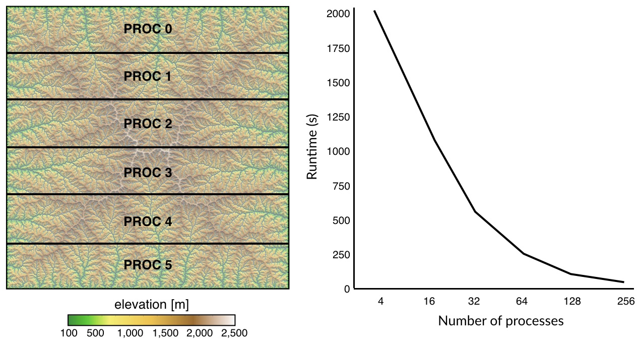
Here we do not perform a parallelisation of the Dijkstra’s algorithm but instead we adopt a simpler strategy where the Dijkstra trees for all paths are balanced and distributed over multiple processors using message passing interface (MPI). The approach consists in splitting the computational domain row-wise as shown in the above figure. Least-cost paths are then computed for the points belonging to each sub-domain using the Dijkstra’s algorithm over the entire region.
Note
Using this approach, LEC computation is significantly reduced and scales really well with increasing CPUs.
| [Bertuzzo2016] | (1, 2, 3) E. Bertuzzo, F. Carrara, L. Mari, F. Altermatt, I. Rodriguez-Iturbe & A. Rinaldo - Geomorphic controls on species richness. PNAS, 113(7) 1737-1742, DOI: 10.1073/pnas.1518922113, 2016. |
| [Dijkstra1959] | E.W. Dijkstra - A note on two problems in connexion with graphs. Numer. Math. 1, 269-271, DOI: 10.1007/BF01386390, 1959. |
| [Etherington2016] | T.R. Etherington - Least-cost modelling and landscape ecology: concepts, applications, and opportunities. Current Landscape Ecology Reports 1:40-53, DOI: 10.1007/s40823-016-0006-9, 2016. |
| [Etherington2017] | T.R. Etherington - Least-cost modelling with Python using scikit-image, Blog, 2017. |
| [Lomolino2008] | M.V. Lomolino - Elevation gradients of species-density: historical and prospective views. Glob. Ecol. Biogeogr. 10, 3-13, DOI: 10.1046/j.1466-822x.2001.00229.x, 2008. |
| [vanderWalt2014] | S. van der Walt, J.L. Schönberger, J. Nunez-Iglesias, F. Boulogne, J.D. Warner, N. Yager, E. Gouillart & T. Yu - Scikit Image Contributors - scikit-image: image processing in Python, PeerJ 2:e453, 2014. |