Quick start guide
I/O Options
The most simple code lines to use bioLEC package is summarised below
import bioLEC as bLEC

biodiv = bLEC.landscapeConnectivity(filename='pathtofile.csv')
biodiv.computeLEC()

biodiv.writeLEC('result')
biodiv.viewResult(imName='plot.png')
Input
The entry point is the function landscapeConnectivity() (see API landscapeConnectivity) that requires the elevation field as it main input.
There are 3 ways to import the elevation dataset :
as a
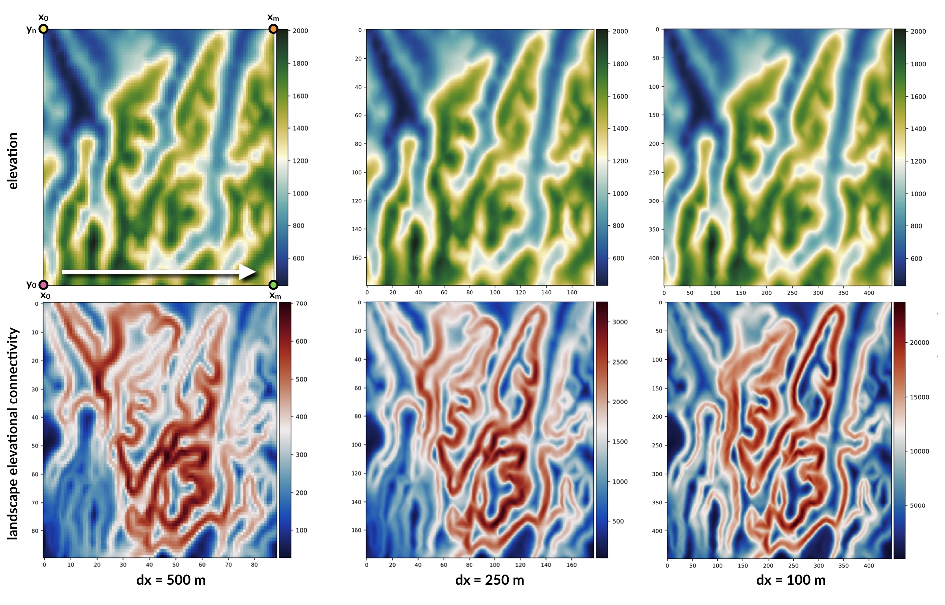
CSVfile (argument:filename) containing 3 columns for X, Y and Z respectively with no header and ordered along the X axis first (as illustrated in the top figure) and shown below:\[\begin{split}\begin{smallmatrix} x_0 & y_0 & z_{0,0} \\ x_1 & y_0 & z_{1,0} \\ \vdots & \vdots & \vdots \\ x_m & y_0 & z_{m,0} \\ x_0 & y_1 & z_{0,1} \\ \vdots & \vdots & \vdots \\ x_m & y_n & z_{m,n} \\ \end{smallmatrix}\end{split}\]as a 3D numpy array (argument:
XYZ) containing the X, Y and Z coordinates here again ordered along the X axis first (as above)or as a 2D numpy array (argument:
Z) containing the elevation matrix (example provided below), in this case thedxargument is also required\[\begin{split}\begin{smallmatrix} z_{0,0} & z_{1,0} & \cdots & z_{m-1,0} & z_{m,0} \\ \vdots & \vdots & \vdots & \vdots & \vdots \\ z_{0,k} & z_{1,k} & \cdots & z_{m-1,k} & z_{m,k} \\ \vdots & \vdots & \vdots & \vdots & \vdots \\ z_{0,n} & z_{1,n} & \cdots & z_{m-1,n} & z_{m,n} \\ \end{smallmatrix}\end{split}\]
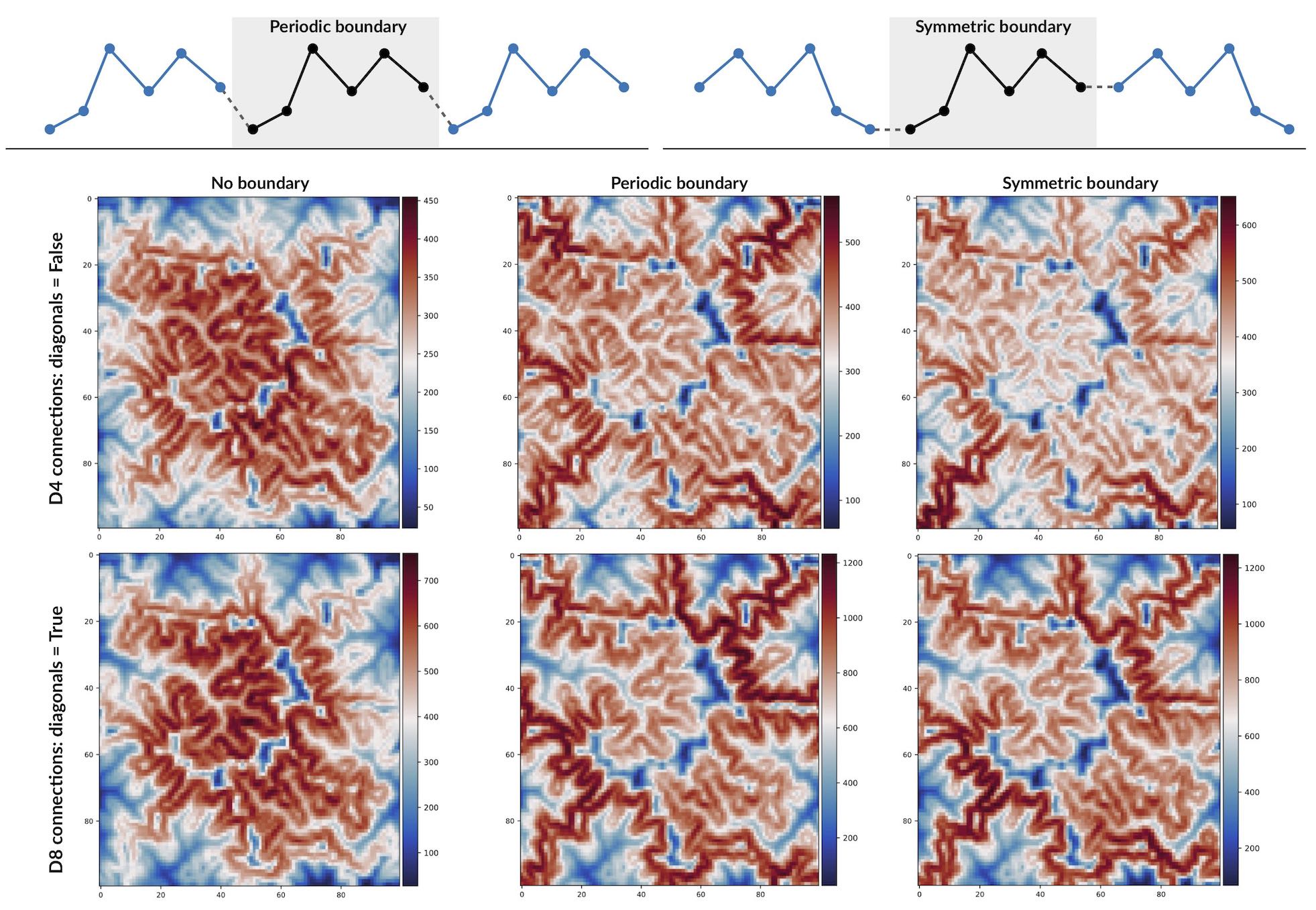
In addition to the elevation field, the user could specify the boundary conditions used to compute the LEC. Two options are available: periodic or symmetric boundaries. The way these two boundaries are implemented in bioLEC is illustrated in the figure below as well as the impact on the LEC calculation.
Finally the LEC solution requires the declaration of the species niche width defined by the variable sigma in the following equation (look in the What is LEC? section for more information):
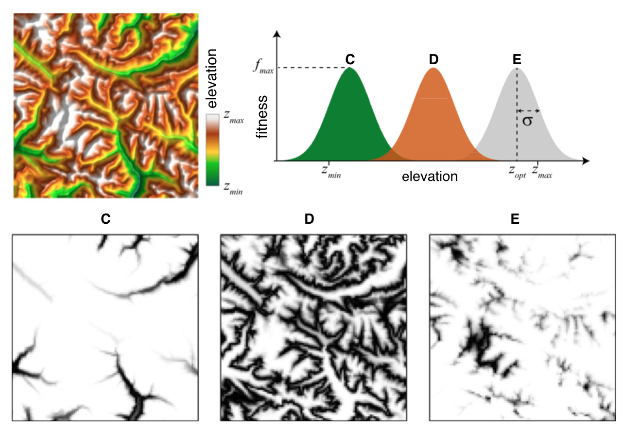
The above figure from [Bertuzzo16] shows the habitat maps as a function of elevation for a real fluvial landscape when considering the fitness of three different species as a function of elevation. The fitness maps of the three species are shown on the bottom panels. In bioLEC two options are possible:
- either the user specifies a species niche width percentage based on elevation extent with the parameter
sigmap - or a species niche fixed width values with the declaration of the parameter
sigmav
Outputs
import bioLEC as bLEC

biodiv = bLEC.landscapeConnectivity(filename='pathtofile.csv')
biodiv.computeLEC()

biodiv.writeLEC('result')
biodiv.viewResult(imName='plot.png')
Once the computeLEC() function (see API compute LEC) has been ran, the result are then available in different forms.
From the writeLEC function (see API write LEC), the user can first save the dataset in CSV and VTK formats containing the X,Y,Z coordinates as well as the computed LEC and normalised LEC (_nLEC_).
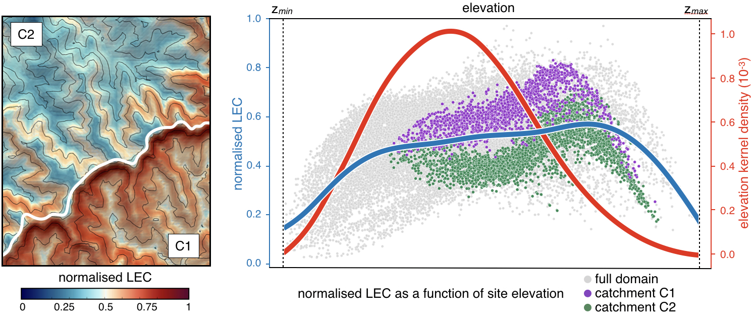
Then several figures can be created showing maps of elevation and LEC values as well as graphs of LEC and elevation frequency as a function of site elevation (such as the figure presented below). In some functions, one can plot the average and error bars of LEC within elevational bands.
Available plotting functions are provided below:
viewResultviewElevFrequencyviewLECFrequencyviewLECZbarviewLECZFrequency
For a complete list of available options, users need to go to the API documentation.
Running examples
There are different ways of using the bioLEC package. If you used a local install with pip, you can download the Jupyter Notebooks provided in the Github repository…
$ git clone https://github.com/Geodels/bioLEC.git
Binder & Docker
The series of Jupyter Notebooks can also be ran with Binder that opens those notebooks in an executable environment, making the package immediately reproducible without having to perform any installation.
This is by far the most simple method to test and try this package, just launch the demonstration at bioLEC-live (mybinder.org)!
Another straightforward installation that again does not depend on specific compilers relies on the docker virtualisation system. Simply look for the following Docker container geodels/biolec.
Note
For non-Linux platforms, the use of Docker Desktop for Mac or Docker Desktop for Windows is recommended.
HPC & Terminal
The tool can be used to compute the LEC for any landscape file as long as the data is available from a CSV file containing 3D coordinates (X,Y,Z) with no header and space delimiter.
Attention
Notebooks environment will not be the best option for large landscape models and we will recommend the use of the python script: runLEC.py in HPC environment.
In this case, the code will be ran from a terminal like this:
$ mpirun -np XX python runLEC.py -i 'xyzfile.csv' -o 'result'
where XX represents the number of processors to use.
The python script runLEC.py is provided in the same folder as the Jupyter notebooks and is defined by:
import argparse
from mpi4py import MPI
import bioLEC as LEC

comm = MPI.COMM_WORLD
size = comm.Get_size()
rank = comm.Get_rank()

# Parsing command line arguments
parser = argparse.ArgumentParser(description='This is a simple entry to run bioLEC package from python.',add_help=True)

# Required
parser.add_argument('-i','--input', help='Input file name (csv file)',required=True)
parser.add_argument('-o','--output',help='Output file name without extension', required=True)

# Optional
parser.add_argument('-p','--periodic',help='True/false option for periodic boundary conditions', required=False, action="store_true", default=False)
parser.add_argument('-s','--symmetric',help='True/false option for symmetric boundary conditions', required=False, action="store_true", default=False)
parser.add_argument('-w','--width',help='Float option for species niche width percentage', required=False, action="store_true", default=0.1)
parser.add_argument('-f','--fix',help='Float option for species niche width fix values', required=False, action="store_true", default=None)
parser.add_argument('-c','--diagonals',help='True/false option for computing the path based on the diagonal moves as well as the axial ones eg. D4/D8 connectivity', required=False, action="store_true", default=True)
parser.add_argument('-n','--nout',help='Number for output frequency during run', required=False, action="store_true", default=500)
parser.add_argument('-d','--delimiter',help='String for elevation grid csv delimiter', required=False,action="store_true",default=' ')
parser.add_argument('-l','--level',help='Float for sea level position', required=False,action="store_true",default=-1.e6)
parser.add_argument('-v','--verbose',help='True/false option for verbose', required=False,action="store_true",default=False)

args = parser.parse_args()
if args.verbose and rank == 0:
  print("Required arguments: ")
  print("   + Input file: {}".format(args.input))
  print("   + Output file without extension: {}".format(args.output))
  print("\nOptional arguments: ")
  print("   + Periodic boundary conditions for the elevation grid: {}".format(args.periodic))
  print("   + Symmetric boundary conditions for the elevation grid: {}".format(args.symmetric))
  print("   + Species niche width percentage based on elevation extent: {}".format(args.width))
  print("   + Species niche width based on elevation extent: {}".format(args.fix))
  print("   + Computes the path based on the diagonal moves as well as the axial ones: {}".format(args.diagonals))
  print("   + Elevation grid csv delimiter: {}".format(args.delimiter))
  print("   + Sea level position: {}".format(args.level))
  print("   + Number for output frequency: {}\n".format(args.nout))

biodiv = LEC.landscapeConnectivity(filename=args.input,periodic=args.periodic,symmetric=args.symmetric,
                                    sigmap=args.width,sigmav=args.fix,diagonals=args.diagonals,
                                    delimiter=args.delimiter,sl=args.level)

biodiv.computeLEC(args.nout)

biodiv.writeLEC(args.output)

if rank == 0:
    biodiv.viewResult(imName=args.output+'.png')
    biodiv.viewElevFrequency(input=args.output,imName=args.output+'_zfreq.png')
    biodiv.viewLECZFrequency(input=args.output,imName=args.output+'_leczfreq.png')
    biodiv.viewLECFrequency(input=args.output,imName=args.output+'_lecfreq.png')
    biodiv.viewLECZbar(input=args.output,imName=args.output+'_lecbar.png')
| [Bertuzzo16] | E. Bertuzzo, F. Carrara, L. Mari, F. Altermatt, I. Rodriguez-Iturbe & A. Rinaldo - Geomorphic controls on species richness. PNAS, 113(7) 1737-1742, DOI: 10.1073/pnas.1518922113, 2016. |